POST ON 2024-03-05 BY WOLVES

UPDATE ON 2025-01-06 BY WOLVES

Deep Learning

You can see the code of this blog on github

1.Neurons and Artificial Neural Networks

Biological Neurons	Artificial Neural Networks
Composed of cell body, dendrites, and axon	Composed of nodes (artificial neurons)
Dendrites receive signals, axon transmits signals	Nodes receive input signals and perform weighted summation
Signals are transmitted through synapses	Signals are transmitted through connections (weights)
Use chemical or electrical signals	Use mathematical functions and algorithms
Complex biological structure	Computational model, divided into input layer, hidden layers, and output layer

This table shows the comparison between biological neurons and artificial neural networks, helping to understand their similarities and differences.

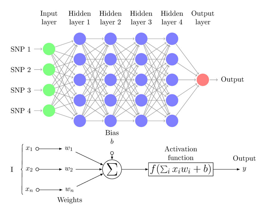
2. Forward Propagation

In a neural network, forward propagation refers to the process of signal transmission from the input layer to the output layer. Each node (neuron) receives input signals, performs a weighted summation, and generates output signals through an activation function. The basic steps of forward propagation are as follows:

1. Input Layer: Receives input data $\vec{x}$.
2. Hidden Layer: Each node calculates the weighted sum $z = \sum (w_i \cdot x_i) + b$, where $w_i$ is the weight and $b$ is the bias.
3. Activation Function: The weighted sum $z$ is passed through an activation function $a = f(z)$ to generate the output.
4. Output Layer: Outputs the final result.

The purpose of forward propagation is to compute the output of the neural network for prediction or classification.

3. Backward Propagation

Backpropagation is a key algorithm used in training neural networks. It involves propagating the error from the output layer back through the network to update the weights and biases, minimizing the error in predictions. The basic steps of backpropagation are as follows:

1. Calculate Error: Determine the error at the output layer by comparing the predicted output with the actual target values.
2. Output Layer: Compute the gradient of the loss function with respect to the output of the network.
3. Hidden Layers: Propagate the error back through the network, calculating the gradient of the loss function with respect to each layer’s weights and biases.
4. Update Weights and Biases: Adjust the weights and biases using the calculated gradients and a learning rate to minimize the error.

The purpose of backpropagation is to optimize the neural network’s parameters, improving its accuracy in making predictions or classifications.

4. Activation Function

Activation functions are used to introduce non-linearity into the neural network, allowing it to handle complex patterns in data. Common activation functions include:

• Sigmoid function: $a = \frac{1}{1 + e^{-z}}$
• ReLU (Rectified Linear Unit): $a = \max(0, z)$
• Tanh (Hyperbolic Tangent):

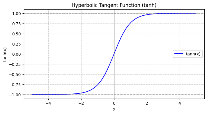
These functions help the neural network learn and generalize better.

4.1 How to choose activation function

• Select the activation function based on the value of y

• The most common activation function is ReLU

• For output layer (In common classification problems)

  • If the value of y is negative or positive, use sigmoid function
  • If the value of y is always equal or greater than 0, use Linear function
  • Relu is not recommended for output layer

• For hidden layer

  • Relu is the most common activation function

5. Multiclass Classification

• from positive and negative to multiple classes

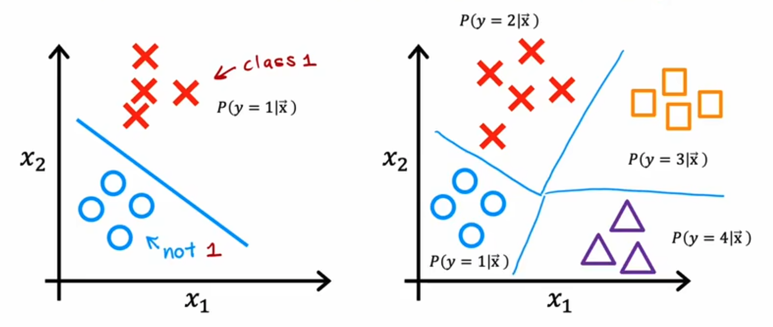
• Now , We need a new activation function to handle multiple classes like softmax function

5.1 Softmax Function

$$ z_i = w_i \cdot x + b_i $$

$$ a_i = \frac{e^{z_i}}{\sum_{j=1}^{n} e^{z_j}} $$

• sparse categorical cross entropy function (稀疏分类交叉熵函数) $$ loss = - \sum_{i=1}^{n} y_i \log(a_i) = - \log(a_{true}) $$

5.2 Numerical RoundOff Error

• Numerical Stability: In calculating the cross-entropy loss (Cross-Entropy Loss), directly inputting logits into the loss function rather than the probability after the sigmoid activation function can improve numerical stability. This helps avoid numerical underflow or overflow issues caused by extreme probability values (close to 0 or 1).

• Use from_logits=True in loss function When setting from_logits=true, the loss function (such as BinaryCrossentropy or CategoricalCrossentropy) automatically applies the sigmoid or softmax activation function internally. Therefore, the last layer of the model only needs to output logits, without manually adding an activation function. This simplifies the model definition and makes the code more concise.

It is equivalent to skipping the intermediate calculation and directly calculating the final result, thereby improving numerical stability.

5.3 RMSProp Optimizer

• 在深度学习中，RMSprop（Root Mean Square Propagation）是一种常用的优化算法，主要用于解决梯度下降中的学习率调整问题。它通过自适应地调整每个参数的学习率，能够有效地加速收敛并减少震荡。

$$ E[g^2]t = \beta E[g^2]{t-1} + (1 - \beta) g_t^2 $$

$$ w_{t+1} = w_t - \frac{\eta}{\sqrt{E[g^2]_t + \epsilon}} g_t $$

5.4 Adam Optimizer (自动选择学习率)

Adam Optimizer

Adam (Adaptive Moment Estimation) is an optimization algorithm that combines the advantages of two other extensions of stochastic gradient descent, namely adaptive gradient algorithm (AdaGrad) and Root Mean Square Propagation (RMSProp). It computes adaptive learning rates for each parameter.

Advantages of Adam Optimizer

• Adaptive Learning Rates: Adam computes individual adaptive learning rates for different parameters from estimates of first and second moments of the gradients.

• Efficient: It is computationally efficient and has low memory requirements.

• Invariance to Diagonal Rescaling of Gradients: The algorithm is invariant to diagonal rescaling of the gradients.

• Suitable for Non-stationary Objectives: It works well with problems that are large in terms of data/parameters or non-stationary.

$$ m_t = \beta_1 m_{t-1} + (1 - \beta_1) g_t $$

$$ v_t = \beta_2 v_{t-1} + (1 - \beta_2) g_t^2 $$

$$ \hat{m}t = \frac{m_t}{1 - \beta_1^t} $$ $$ \hat{v}t = \frac{v_t}{1 - \beta_2^t} $$

$$ w_{t+1} = w_t - \frac{\eta}{\sqrt{\hat{v}_t} + \epsilon} \hat{m}_t $$

6.Some Concepts

6.1 Parameter & Hyperparameter

• Parameter: The weights and biases in the model

• Hyperparameter: The learning rate, batch size, number of epochs, etc.

• In the training process, the model parameters are adjusted through backpropagation, while the hyperparameters are set manually by the user.

• Maybe we can use some methods to find the best hyperparameter in the future, but now we can only set it by experience.

6.2 human brain and deep learning

There are many similarities between the human brain and deep learning. Deep learning models are inspired by the structure and function of the human brain, particularly the way neurons and synapses work. But today, deep learning models are still far from the complexity and flexibility of the human brain.

• Neurons and Artificial Neurons: The human brain is composed of billions of neurons connected through synapses. Similarly, deep learning models consist of many artificial neurons connected by weights.

• Learning Process: The human brain continuously adjusts the strength of connections between neurons through experience and learning. Deep learning models adjust weights using training data and backpropagation algorithms to minimize the loss function.

• Hierarchical Structure: Neurons in the human brain are distributed across different regions and layers, responsible for processing different types of information. Deep learning models also consist of multi-layer neural networks, with each layer extracting different levels of features.

Although deep learning models perform excellently on certain tasks, they are still far from the complexity and flexibility of the human brain. Future research may further draw on the principles of the human brain to enhance the performance and adaptability of deep learning models.

6.3 train/dev/test sets

In the begnning of DL, we need to define the number of layers, hidden units, learning rate, activation function, etc(hyperparameter).

• train set: used for training the model
• dev set: used for tuning the model
• test set: used for testing the model

6.4 vanishing/exploding gradient

• the gradient is too small, especially in the hidden layer which uses sigmoid/tanh activation function
  • the gradient is too small, so the model will not learn anything
  • the model will be stuck in the local minimum
• the gradient is too large, especially in the hidden layer which uses ReLU activation function
  • the gradient is too large, so the model will explode
  • the model will be unstable

6.5 weight initialization

• random initialization
• He initialization - for ReLU activation function $$W \sim \mathcal{N}(0, \sqrt{\frac{2}{n_{in}}})$$
• Xavier initialization - for sigmoid/tanh activation function $$W \sim \mathcal{N}(0, \sqrt{\frac{1}{n_{in}}})$$

$n_{in}$ 表示当前层的输入神经元数量

6.6 mini-batch gradient descent

• mini-batch gradient descent is a variant of gradient descent that uses a small subset of the training data (mini-batch) to update the model parameters.

• It is used to speed up the training process and reduce the memory usage.

• Advantages

  • lower memory usage
  • faster convergence
  • better generalization

• eg. Data set has 10000 samples, we will use 100 of them to update the model parameters at one time

6.7 Gradient Checking

• Gradient Checking is a technique used to verify the correctness of the gradient calculation in the backpropagation algorithm.
• It is used to check whether the gradient calculated by the backpropagation algorithm is correct.
• It is used to check whether the gradient calculated by the backpropagation algorithm is correct.

7. Bias and Variance

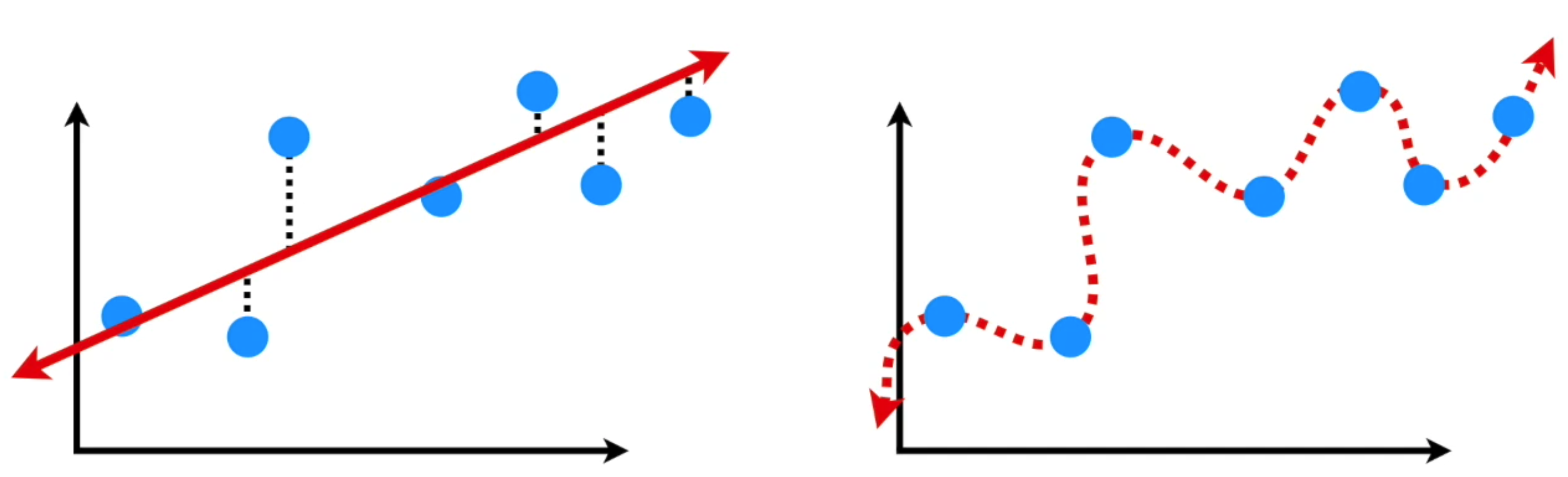
• In this case

  • the left is the high bias, the right shows a low bias
  • the left is the low variance, the right shows a high variance
  • And the left is a overfitting model, the right is a underfitting model

• Bias: The difference between the expected value and the true value

• Variance: The difference between the predicted value and the expected value

8. Regularization

• Regularization is a technique used to prevent overfitting in deep learning models. It adds a penalty term to the loss function to encourage the model to learn simpler patterns.

• L1 Regularization: $loss = loss + \lambda ||w||_1$

• L2 Regularization: $loss = loss + \lambda \sum w^2$

• (L2 Regularization is also called weight decay)

• $\lambda$ is the regularization parameter, which controls the strength of the regularization.

8.1 Dropout

• Dropout is a regularization technique that randomly drops out some neurons during training to prevent overfitting.

• During each training iteration, different neurons may be randomly deactivated, which enhances the learning strength of other neurons and improves the model’s generalization ability.

8.2 Other Regularization Techniques

• Early Stopping

9.Computer Vision

From this part, we will learn how to use DL to solve some problems in computer vision.

9.1 Some problems

• Instead of using 64x64x3 to represent an image, we may face 1000x1000x3 to represent an image, it means the input layer will possess a lot of parameters, which will cost a lot of time and memory in calculation.

• So we need to use some methods to reduce the dimension of the input layer.

9.2 Some concepts

• Gray Image
  • Every pixel has only one channel, it just represents the brightness of every pixel
  • the value range is [0,255]
  • It`s always used in margin detection or binary classification
• RGB Image
  • Every pixel has three channels, it represents the brightness of every pixel in the red, green and blue channels
  • the value range is [0,255]
  • It`s always used in object detection or multi-class classification

9.3 SVM

• Support Vector Machine is a type of machine learning algorithm that is used for classification and regression.

10 Convolutional Neural Network

• Convolutional Neural Network (CNN) is a type of neural network that is commonly used in computer vision tasks.

• It is a type of feedforward neural network that is specifically designed for image processing and analysis.

• it will reduce the parameters and the calculation of the model, it also can extract the features of the image

10.1 Edge detection

• use a 3x3 filter to detect the edge of the image

• filters

  • Sobel filter
    • $G_x = \begin{bmatrix} -1 & 0 & 1 \ -2 & 0 & 2 \ -1 & 0 & 1 \end{bmatrix}$
    • $G_y = \begin{bmatrix} -1 & -2 & -1 \ 0 & 0 & 0 \ 1 & 2 & 1 \end{bmatrix}$
  • Prewitt filter
    • $G_x = \begin{bmatrix} -1 & 0 & 1 \ -1 & 0 & 1 \ -1 & 0 & 1 \end{bmatrix}$
    • $G_y = \begin{bmatrix} -1 & -1 & -1 \ 0 & 0 & 0 \ 1 & 1 & 1 \end{bmatrix}$
  • Scharr filter
    • $G_x = \begin{bmatrix} -3 & 0 & 3 \ -10 & 0 & 10 \ -3 & 0 & 3 \end{bmatrix}$
    • $G_y = \begin{bmatrix} -3 & -10 & -3 \ 0 & 0 & 0 \ 3 & 10 & 3 \end{bmatrix}$

• then, we use the filter with the part of the image to calculate the convolution,we will get a new image(feature map), which is smaller than the original image

• the result of the convolution will enhance the edge of the image

10.2 Padding

• Padding is a technique used to keep the size of the image after the convolution

• when we process a 6x6 image with a 3x3 filter, we will get a 4x4 feature map, because the filter can only move 4x4 times in the image

• the peak pixel will use a little part of the image, which will cause the loss of information

• so we need to use padding to keep the size of the image, it will add a border around the image and the peak pixel will use more to express the information

  • $n_{out} = \frac{n_{in} - n_{filter} + 2 \times padding}{stride} + 1$
  • $n_{out}$ is the output size
  • $n_{in}$ is the input size
  • $n_{filter}$ is the filter size
  • $padding$ is the padding size
  • $stride$ is the stride size

10.3 Stride

• Stride is the step size of the filter when moving in the image

• when we use a 3x3 filter to process a 6x6 image, we will get a 4x4 feature map, because the filter moves 1 pixel each time

• we can also use 2 stride to reduce the size of the feature map

10.4 three dimensions

• RGB image - 三层堆叠

  • 3 channels
  • 3x3x3 filter
  • 3x3x3 feature map

• The same example 6x6 image with 3 channels, the filter will be 3x3x3 which like a cube. then use the every layer of the filter to process the every layer of the image part by part, and then we will get a 4x4x3 feature map, then add them together, we will get a 4x4x1 feature map.

10.5 One layer of a Convolutional Neural Network

卷积核+偏置+激活函数+(其他)

• In the previous part, we use a 3x3x3 filter to process a 6x6x3 image to get the single feature map, but in the real situation, we need to use many filters to process the image, and then we will get many feature maps and then stack them up.

• The result is like this:

  • 6x6x3 image

  • 3x3x3 filter

  • 3x3x3 filter

  • 4x4x2 feature map

• And that is the one simple layer of a Convolutional Neural Network.

• Here is a case:

  • 6x6x3 image
  • 10 filters with 3x3x3

• the output will be:

  • 4x4x10 feature maps
  • (3x3x3 + 1)x10 parameters (We alse have a bias ‘b’ for each filter)

• In this case, the model will not easy to overfit, because the number of parameters is not too large, we can use more filters to process a image which is very complex and huge.

10.6 Convolutional Neural Network

• we can use many layers to process the image, and then we will get a more complex and huge feature map, then unrolling them into a very long vector, use the logistic regression or softmax regression to process it which like a normal neural network, and that is the Convolutional Neural Network.

10.7 Pooling layer

• Pooling layer is a layer that uses a filter to process the image for reducing the size of the feature map

• The most common pooling is max pooling, it will select the maximum value in the filter’s range, and then we will get a new feature map, which is smaller than the original feature map.

• The result of the pooling is like this:

  • original 4x4x10 feature maps
  • result 2x2x10 feature maps

• Pooling is alse a filter, but it will not multiply the weight and the bias, it will just select the maximum value in the filter’s range, and it will keep the same number of channels.

• There is another pooling is average pooling, it will select the average value in the filter’s range.

10.8 Fully Connected Layer

• The Fully Connected Layer (FC Layer) is a common type of layer in neural networks, typically used to map the output from the previous layer to the final prediction result.

• Like the normal machine learning, we can use many FC layer to process the image, and then we will get a very long vector, and then use the logistic regression or softmax regression to process it which like a normal neural network.

10.9 Hyperparameter

• Hyperparameter is a parameter that is not learned from the data, it is set by the user.

• We can get the best hyperparameter by looking papers or using some tools instead of ourselves.

11. classic network

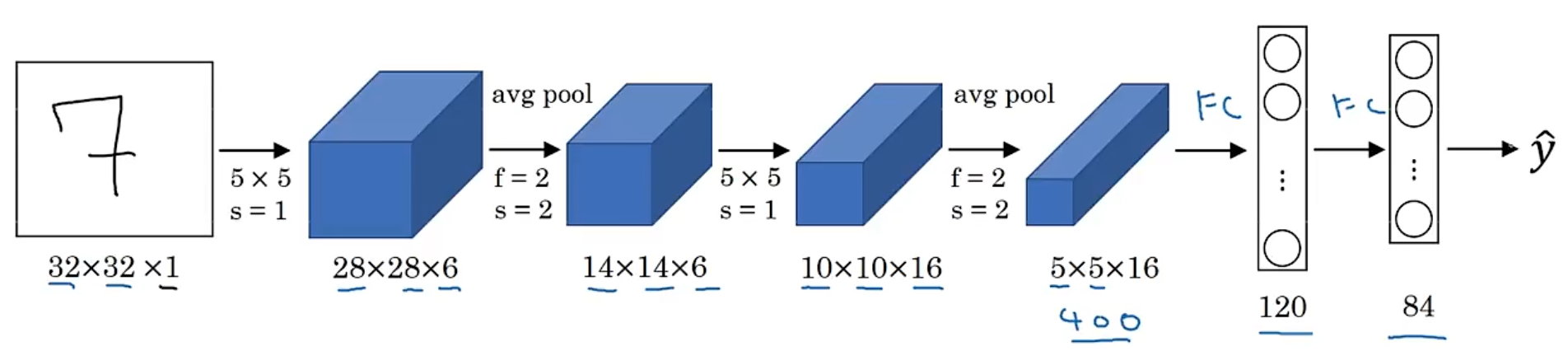
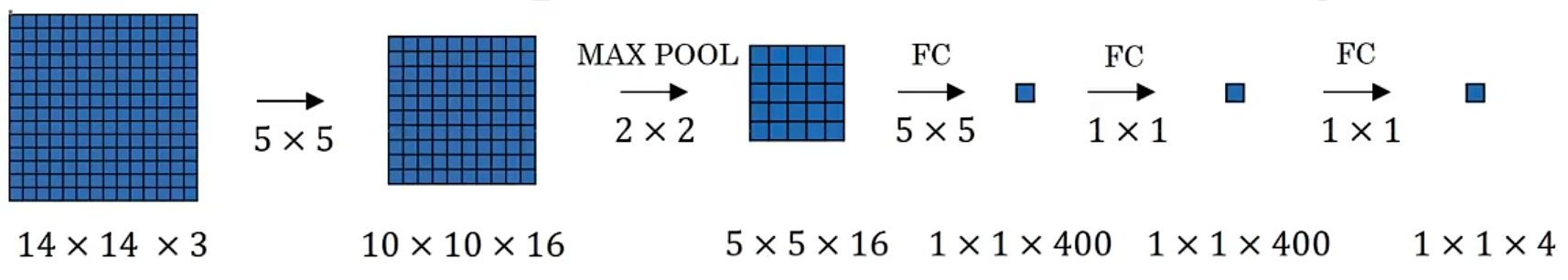
11.1 LeNet-5

• LeNet-5 is a classic network in the field of computer vision, which is used for handwritten digit recognition.

• You can use max pooling install of average pooling.

• It has more than 60000 parameters, it is very small than the modern network.

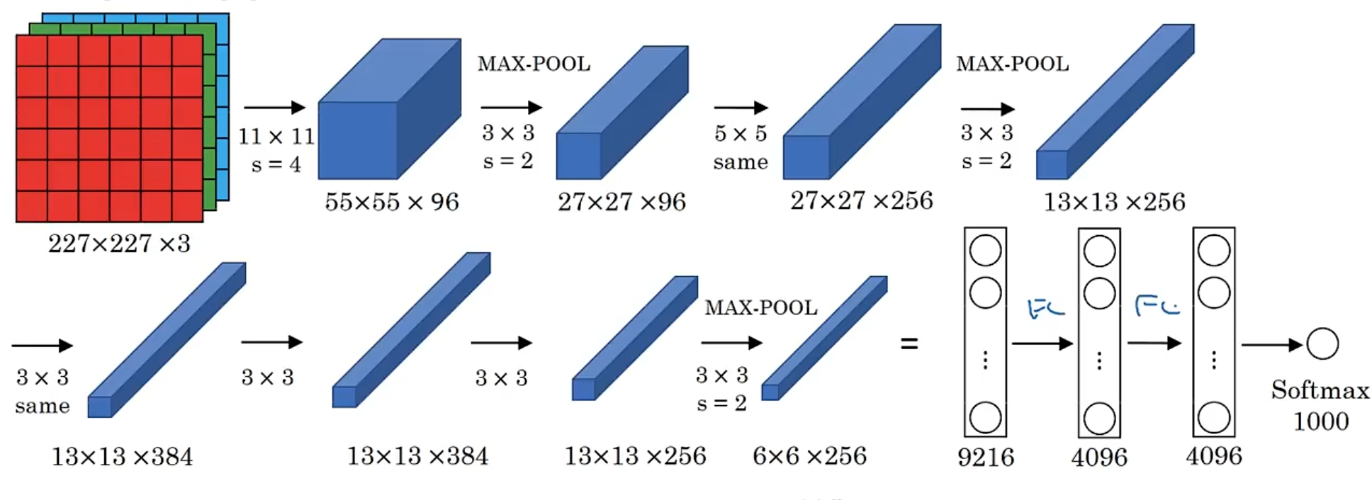
11.2 AlexNet

• AlexNet is a classic network in the field of computer vision, which is used for image classification.

• It has more than 60m parameters

• Local Response Normalization (LRN) - normalize the feature map channel by channel

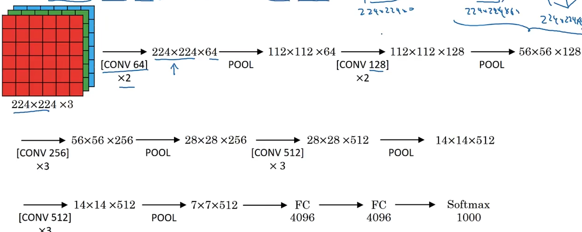
11.3 VGG

• VGG is a classic network in the field of computer vision, which is used for image classification.

• It has more than 138m parameters

• 3x3 filter with 1 stride

• 2x2 max pooling with stride 2

11.4 GoogleNet

• GoogleNet is a classic network in the field of computer vision, which is used for image classification.

• It has more than 60m parameters

• 3x3 filter with 1 stride

• 2x2 max pooling with stride 2

• It use padding to keep the size of the feature map

• Vgg16 has more than 138m parameters

• Vgg19 has more than 140m parameters

12. Modern Network

12.1 ResNet

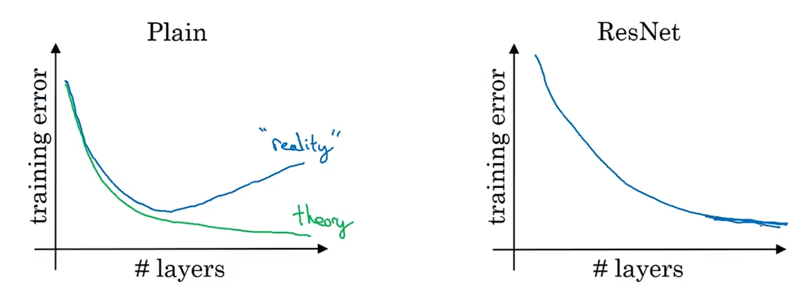
• Every depp neural network are difficult to train becase of vanishing and exploding gradient.

• The function of ResNet is to use a skip connection to solve the problem of vanishing and exploding gradient, which allows you to take the activation from one layer and suddenly feed it to another layer.

12.1.1 Residual Block

• It didn’t follow the main path of the network, it use a [skip connection](shortcut) pass one or more layers for going much deeper.

• eg.

before:

$$a^{[l+2]} = g(z^{[l+2]}) = g(W^{[l+2]}a^{[l+1]} + b^{[l+2]})$$

after:

$$a^{[l+2]} = g(z^{[l+2]} + a^{[l]}) = g(W^{[l+2]}a^{[l+1]} + b^{[l+2]} + a^{[l]})$$

• The normal path is $a^{[l+2]} = g(z^{[l+2]})$ and the path with the layer it skip is a Residual Block.

12.1.2 ResNet

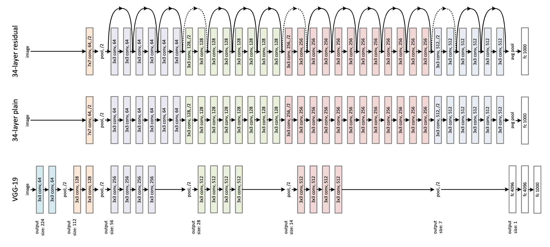
• The dashed lines in the figure indicate that the dimensions on both sides of skip connction are different and special processing is required

12.1.3 1x1 Convolution

• 1x1 Convolution is a type of convolution that is used to change the dimension of the feature map

• It is used to reduce the number of parameters and the calculation of the model

• It likes a full connection layer, but it is used in the convolutional layer

• In practice, we will employ a pooling layer to reduce the dimensionality of the feature map, followed by a 1x1 convolution to alter the channel configuration of the feature map.

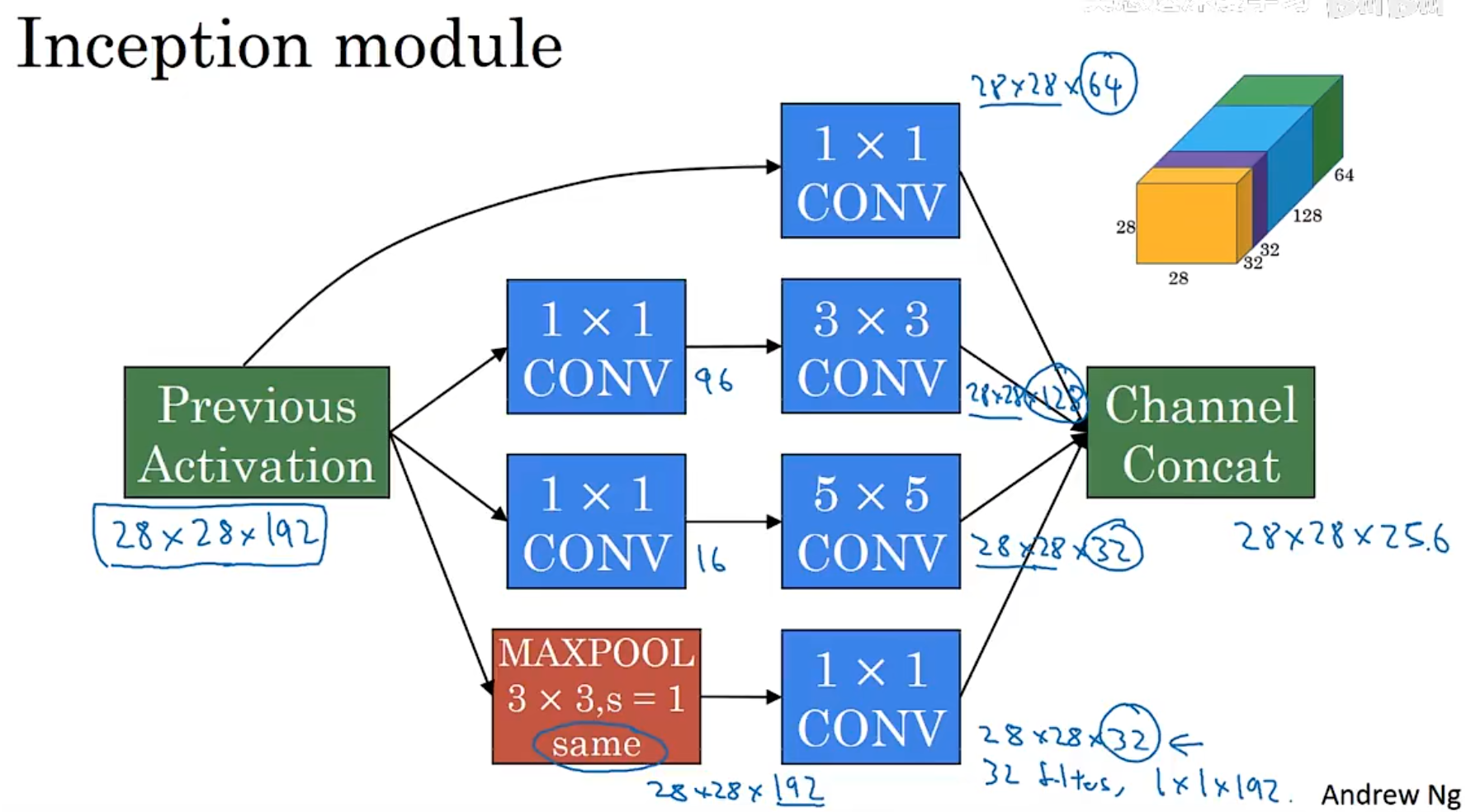
12.1.4 Inception Network

• Inception Network is a collection of different layers. we don’t know which layer is the best, we just use all of them and merge them together into a new feature map.

• Inception Network use parallel structure to process the image, it uses a convolution kernels of different sizes (e.g. 1x1, 3x3, 5x5) in the same layer enables simultaneous extraction of local details and global context information

输入
├── 1x1x64 卷积
├── 3x3x128 卷积 → 3x3 卷积
├── 5x5x32 卷积 → 5x5 卷积
└── 3x3x32 最大池化 → 1x1 卷积
输出（拼接所有分支的结果）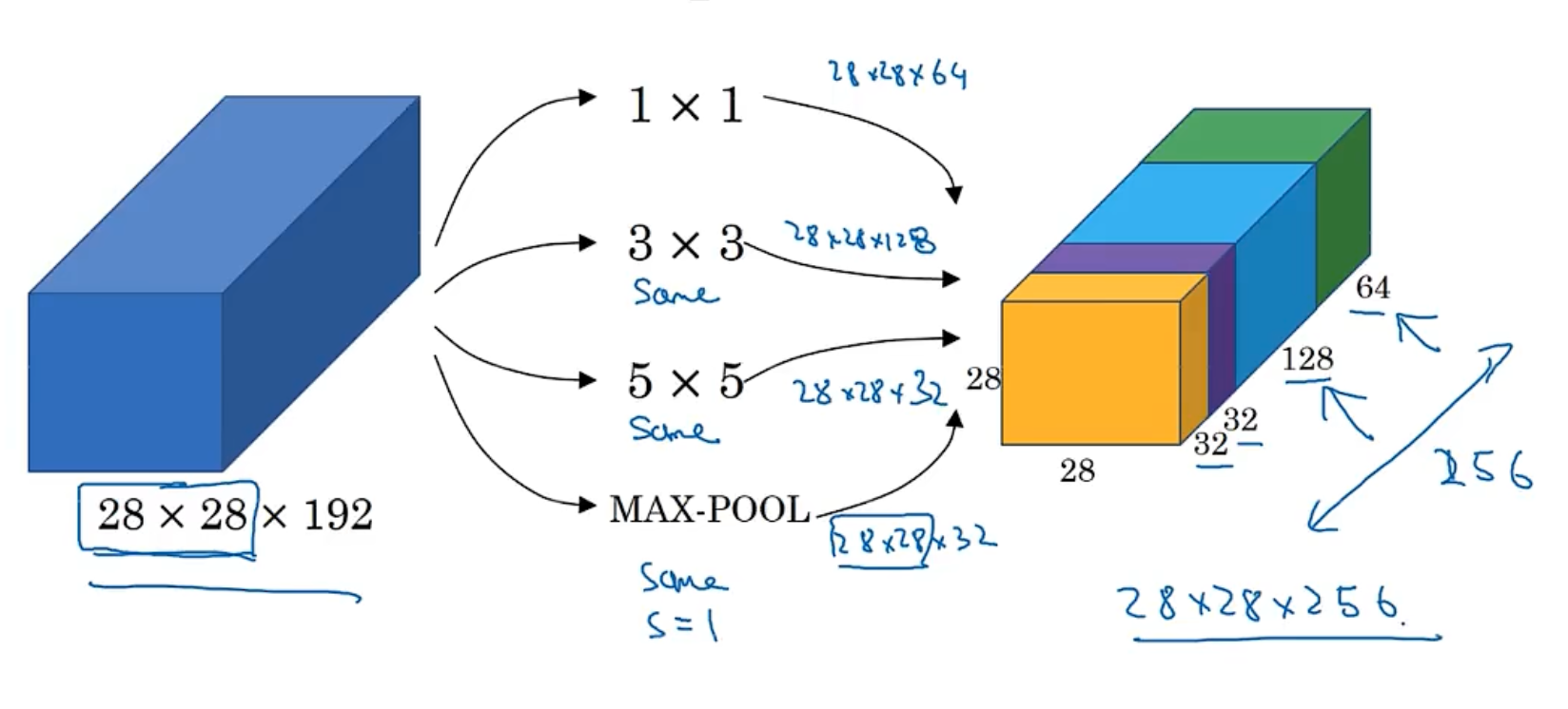

• But the Inception Network has a lot of parameters, the scale of computation is too huge. To address this issue, we can use 1x1 convolution to reduce the number of channels. It will reduce an order of magnitude.

13. Transfer Learning

• There is a huge amount of case which has been trained by others, we can use the pre-trained model to solve a new problem.

• The new layer will learn the new feature, and the pre-trained layer will still learn the old feature.

• The greater the influx of new data, the more layers you can replace.

14. Object Detection

Image Classification -> Classification with locatization -> Object Detection

14.1 Classification with locatization

• The output will not only the classification result, but also the locatization result - bounding box.

• the datset need to provide the bounding box of the object, not only the detected object, but also the background.

• Sliding Window Detection

• The sliding window will slide over the image, and then use the classification model to classify the image.

• The bounding box will be the same size, so it will be very slow. And It gets bigger every round.

• In this case, the bounding box is not accurate, and it is not a good result even it can not detect the object.

14.2 landmark detection

• landmark detection is a technique that detects the landmark of the object, such as the eyes, mouth, nose, etc. It will provide the key points of the object.

• It can be used in the face detection, the object detection, the pose estimation, etc.

14.3 Yolo

• Yolo is means You Only Look Once, it is a method that can detect the object in the image.

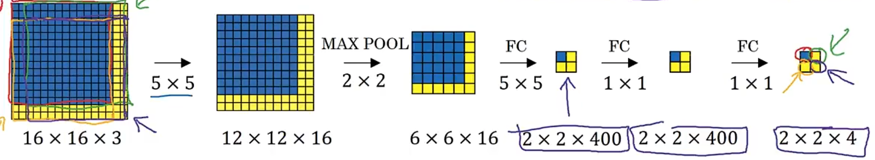
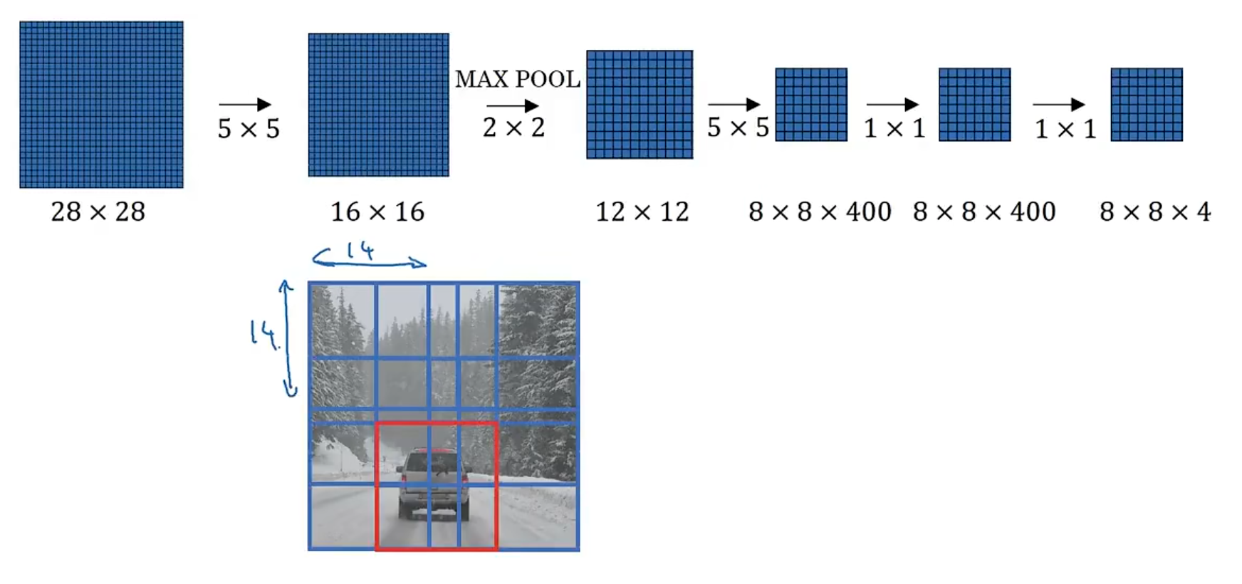
• First, we need to divide the image into a grid

• Then, For each grid, we need to predict the bounding box of the object and the class of the object.

• It will use a key point to represent the object, and the key point will be the center of the object, yolo use this point to distribute the object to the grid.

• it will output S x S x (bounding box + class), and it is a matrix. (S is the number of grids)

14.4 Intersection Over Union

• Intersection Over Union is a metric that is used to evaluate the performance of the object detection model.

• It is the ratio of the intersection area to the union area of the predicted bounding box and the ground truth bounding box.

• “Correct” if IoU > 0.5, it is just a personal defined threshold.

  • The IoU is the ratio of the intersection area to the union area of the predicted bounding box and the ground truth bounding box.

14.5 Non-max suppression

• Non-max suppression is a technique for making sure that your algorithm detects each object only once.

• In a specific grid, there may be multiple bounding boxes, we maybe check it more than one time

• So, we use Non-max suppression to make sure that the algorithm detects each object only once.

• It will choose the eligible confidence score bounding box, and then suppress the other bounding box with the lower confidence score.

14.6 Anchor Box

• Anchor Box is a technique that is used to detect the object in the image.

• It will use a bounding box to detect the object, and then use the anchor box to detect the object.

14.7 R-CNN (regions with CNN)

• It picks a few regions that makes sense to run conv net classifier.

• We use a segmentation algorithm find blob points, it will find the prominent area of the image, and then we can use conv net to process it.

• 根据分割出的尺度，选择合适的区域，然后进行卷积运算。

• 优点

  • 准确性高

• 缺点

  • 速度慢
  • 计算量大

• Fast R-CNN

  • 使用卷积运算，而不是滑动窗口
  • 使用RoI池化，而不是全连接层，将候选区域映射到特征图上
  • 使用多任务损失函数，而不是单独的分类损失函数

• Faster R-CNN

  • 使用RPN网络，而不是选择性搜索，滑动搜索框，生成候选区域
  • 使用锚框，而不是选择性搜索

15. Face Recognition

• 1.Detect the face
• 2.Detect live or not

15.1 Conceptions

15.1.1 Face Verification vs. face recognition

• Face Verification

  • input: image, face image
  • output: whether is the same person

• Face Recognition

  • input: Has a database of K person
  • get a new image
  • output: judge which person

15.2 One-shot learning

• If we use cnn, it will be not work, because we just have a little data, it is not enough to train a good model. And if there is a new person, we need re-train the model.

• similarity function

  • $d(img1, img2) = degree of difference$
  • if $d(img1, img2) < \delta$, then they are the same person

15.3 Siamese Network

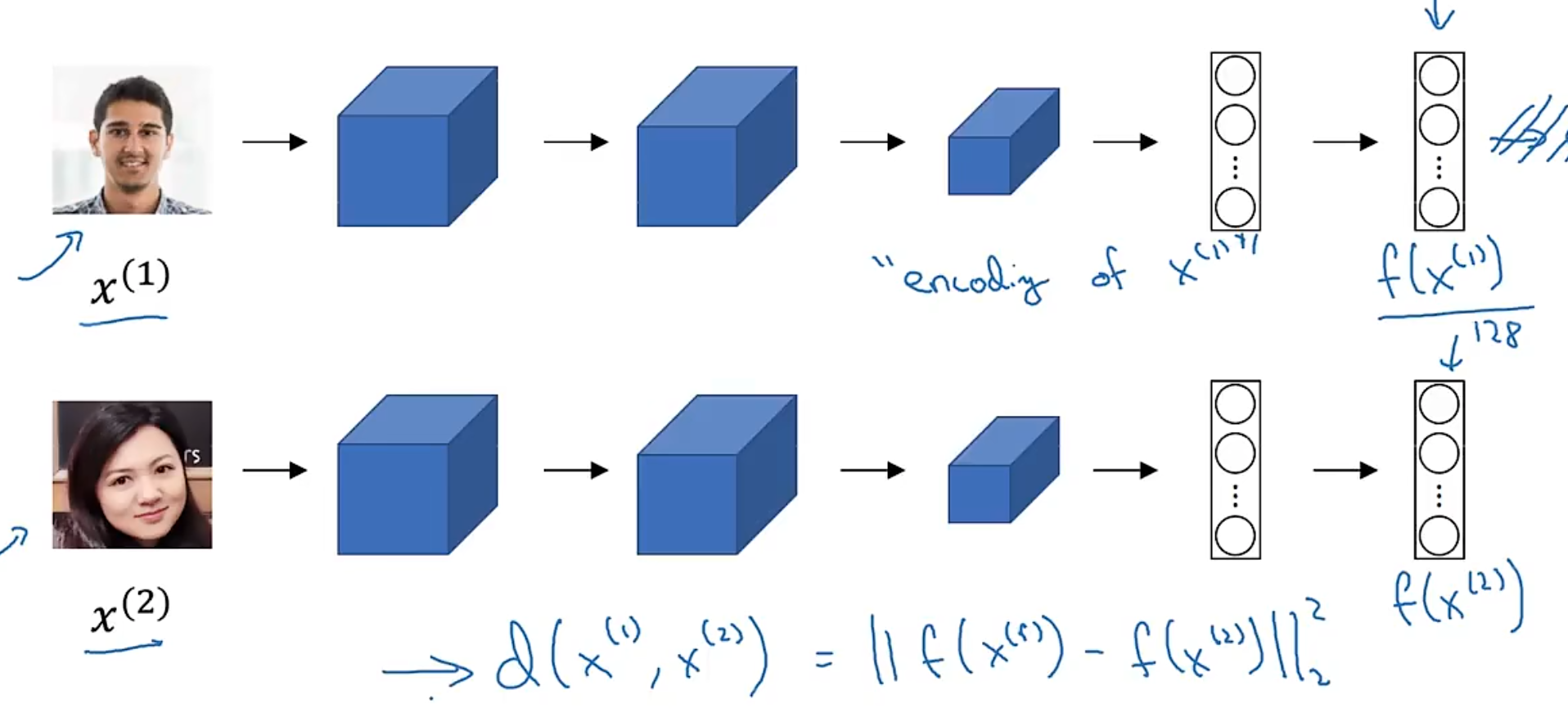
$$d(x^{(1)}, x^{(2)}) = ||f(x^{(1)}) - f(x^{(2)})||^2$$

• if the result is small, then they are the same person

15.4 Triplet Loss

• Anchor, Positive, Negative

• Anchor: the image of the person

• Positive: the image of the same person

• Negative: the image of the other person

• want: $||f(Anchor) - f(Positive)||^2 - ||f(Anchor) - f(Negative)||^2 + \alpha \leq 0$

• so the formula is:

$$L = \max(0, ||f(Anchor) - f(Positive)||^2 - ||f(Anchor) - f(Negative)||^2 + \alpha)$$

$$ I = \sum_{i=1}^{m} L(a^{(i)}, p^{(i)}, n^{(i)}) $$

• we will need a lot of data to train the model, And the relations between Anchor, Positive, Negative is not eays to define, it is difficult to train on.

15.5 Face Recognition

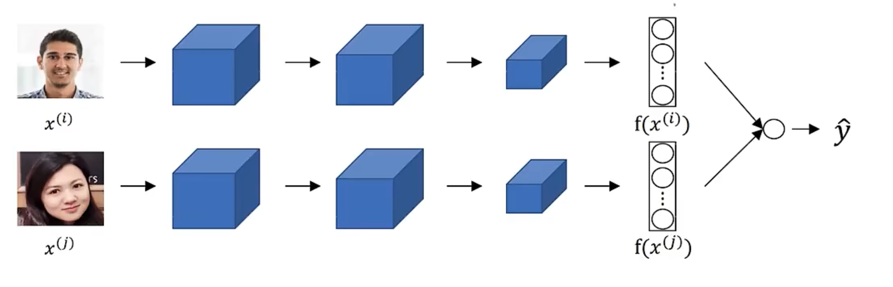
$$ \hat{y} = \sigma(\sum_{k=1}^{k}w_i|f(x^{(i)})_k - f(f^{(j)})_k| + b) $$

or

$$ \hat{y} = \sigma(\sum_{k=1}^{k}w_i\frac{(f(x^{(i)})_k - f(f^{(j)})_k)^2}{f(x^{(i)})_k + f(f^{(j)})_k} + b) $$

• $w_i$ is the weight of the feature
• $b$ is the bias
• $\sigma$ is the sigmoid function

16. Neural Style Transfer

• Neural Style Transfer is a technique that is used to transfer the style of one image to another image.

• It will use a content image and a style image, and then use a neural network to transfer the style of the style image to the content image.

• cost function

$$ J(G) = \alpha J_{content}(C, G) + \beta J_{style}(S, G) $$

• $J(G)$ is the cost function

• $J_{content}(C, G)$ is the cost function of the content image

• $J_{style}(S, G)$ is the cost function of the style image

• content cost function

$$ J_{content}(C, G) = \frac{1}{2}||a^{(C)} - a^{(G)}||^2 $$

• $a^{(C)}$ is the content of the content image

• $a^{(G)}$ is the content of the generated image

• style cost function

$$ J_{style}(S, G) = \sum_{l} \lambda^{[l]} J^{[l]}_{style}(S, G) $$

• $J^{[l]}_{style}(S, G)$ is the cost function of the style image
• $\lambda^{[l]}$ is the weight of the style image

17. Sequence Models

from this part, we will learn how to use RNN, LSTM, GRU to deal with NLP(Natural Language Processing) problems.

• Speech Recognition
• Music Generation
• Sentiment Classification
• Machine Translation
• Video Character Recognition
• Name Entity Recognition

17.1 Notation

• $x^{(i)}$ is the t-th word of the i-th sentence
• $y^{(i)}$ is the t-th word of the i-th sentence

17.2 Math symbols

• motivating example

x : “I want to have a big house in the future”

y : “0 0 0 0 0 1 1 0 0 0”

分别对应$x^{(i)}$和$y^{(i)}$,这指明这个序列的长度是10以及对应标签

• vocabulary

$$V = {a, big, house, in, the, future, i, want, to, have, \cdots }$$

this dictionary maybe has 10000 words, so the size of the vocabulary is 10000, it is very small for today’s standard.

$x^{(i)}$ is the t-th word of the i-th sentence, and it is a one-hot vector, the size of the one-hot vector is the size of the vocabulary.eg. $x^{(i)<1>}$ is ${0, 0, 0, 0, 0, 0, 0, 1, 0, 0, \cdots }$

$y^{(i)}$ 即为强调内容或者是需要预测的内容

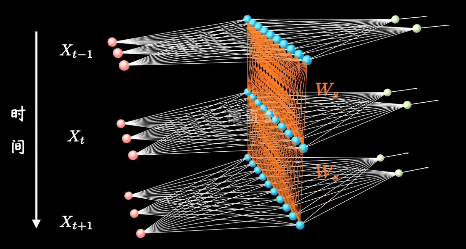
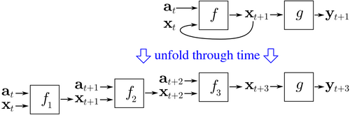
17.3 Recurrent Neural Network

• In previous neural network, if we use the same network to deal with different input, it will be not work, because the size of the input is different too, we can’t train it. Even more, It doesn’t share features learned across different positions of text;

• Recurrent Neural Network is a type of neural network that is used to deal with sequence data.

17.3.1 basic RNN model

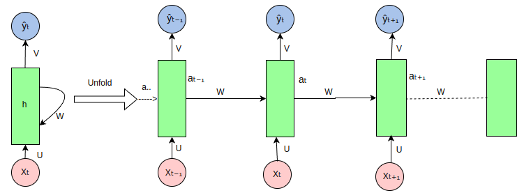
• It means the output of the previous layer is the input of the next layer.

$$ a^{(t)} = \sigma(W_a[a^{(t-1)}, x^{(t)}] + b_a) $$

$$ y^{(t)} = \sigma(W_y[a^{(t)}] + b_y) $$

• $a^{(t)}$ is the hidden state of the t-th word

• $x^{(t)}$ is the t-th word

• $y^{(t)}$ is the output of the t-th word, always is probability or one-hot vector for different solutions

• $W_a$ is the weight of the hidden state

• $a-\sigma$ is always tanh or relu

• $y-\sigma$ is always sigmoid

• $a^{(0)}$ is the initial hidden state, it is a zero vector

• $a^{(t)}$ is the hidden state of the t-th word

• $[a^{(t-1)}, x^{(t)}]$ is the input of the t-th word and overlay them.

17.3.2 Backpropagation through time (BPTT)

• loss function

$$ \frac{1}{T}\sum_{t=1}^{T}L^{(t)}(\hat{y}^{(t)}, y^{(t)}) $$

• $L^{(t)}$ is the loss function of the t-th word

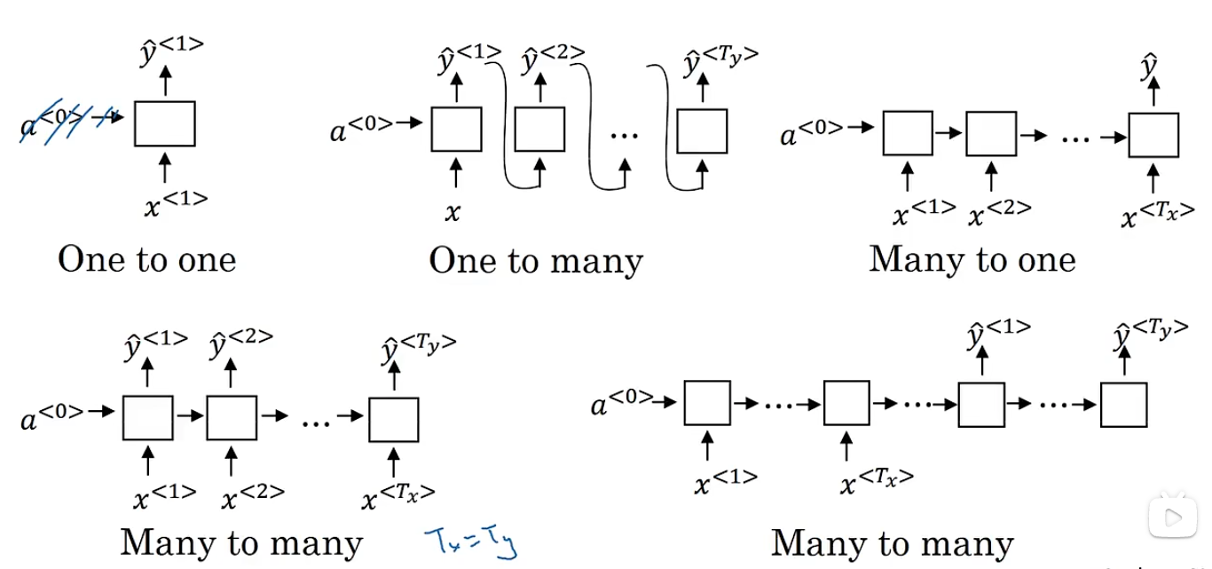
17.3.3 Different types of RNNs

• many to many - many inputs and many outputs - same length
• many to one - many inputs and one output (last output) - classification
• one to many - one input and many outputs - generation
• one to one - one input and one output - classification

17.4 Language model and sequence generation

17.4.1 Language model

• Speech recognition

  • give a sentence, and then predict the probability of the sentence

• Language model

  • <EOS> is the end of the sentence
  • 可以把上一状态的输出作为下一状态的输入
  • 如我输入hello，他先把hell作为输入依次更新rnn的状体并且舍去输出，当输入o的时候，产出一个空格，再把空格变为当前的状态的输入写进去，依次这么做直到出现eos或者length上限

17.4.2 vanishing gradients

• RNN is not good at dealing with long sequences, because the gradient will vanish or explode.

$$ L = \sum_{t=1}^T L_t = -\sum_{t=1}^T y_t \log \hat{y}_t $$

• $L_t$ is the loss function of the t-th word
• $y_t$ is the one-hot vector of the t-th word
• $\hat{y}_t$ is the output of the t-th word

17.4.3 Gated Recurrent Unit (GRU)

• 门控循环单元
• 增强长序列记忆
• 缓解梯度消失问题

时间步 t 的计算：
         ↗ h_{t} = tanh(W_h h_{t-1} + W_x x_t + b)
        /
h_{t-1} → [RNN Cell] 
        \
         ↘ 可能输出 y_t（如分类任务）

• 更新门 - 能关注的机制
• 重置门 - 能遗忘的机制

$$ R_t = \sigma(W_r[h_{t-1}, x_t] + b_r) $$

$$ Z_t = \sigma(W_z[h_{t-1}, x_t] + b_z) $$

$$ \tilde{h}t = \tanh(W_h[R_t \odot h{t-1}, x_t] + b_h) $$

$$ h_t = Z_t \odot h_{t-1} + (1 - Z_t) \odot \tilde{h}_t $$

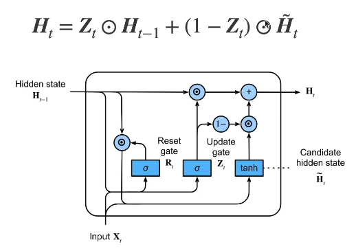
• 实际使用中，尽量使用GRU和LSTM，虽然他们比RNN增加了计算，但是效果会更好

17.4.4 Long Short-Term Memory (LSTM)

• 长短期记忆网络

• 增强长序列记忆

• 缓解梯度消失问题

• 遗忘门 - 决定要不要保留上一个状态的信息

• 输入门 - 决定要不要忽略掉输入的数据

• 输出门 - 决定是不是使用隐藏状态

$$ I_t = \sigma(W_i[h_{t-1}, x_t] + b_i) $$

$$ F_t = \sigma(W_f[h_{t-1}, x_t] + b_f) $$

$$ O_t = \sigma(W_o[h_{t-1}, x_t] + b_o) $$

$$ \tilde{C}t = \tanh(W_c[h{t-1}, x_t] + b_c) $$

$$ C_t = F_t \odot C_{t-1} + I_t \odot \tilde{C}_t $$

$$ h_t = O_t \odot \tanh(C_t) $$

$$ y_t = \sigma(W_y[h_t, C_t] + b_y) $$

• $I_t$ 是输入门
• $F_t$ 是遗忘门
• $O_t$ 是输出门
• $\tilde{C}_t$ 是候选记忆单元
• $C_t$ 是当前记忆单元
• $h_t$ 是隐藏状态
• $y_t$ 是输出

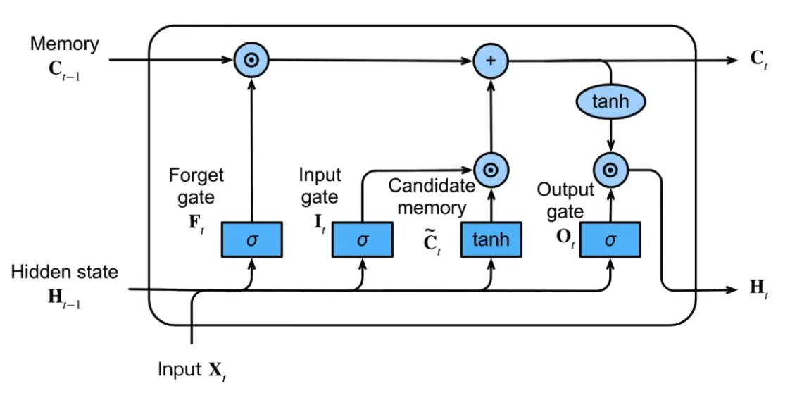
• 相当于是多了$C_t$这么一个新的状态，可以理解为专门用来记忆长期信息，然后当前状态$h_t$根据两者进行融合

• LSTM和GRU在信息的记忆和遗忘上都很灵活

17.5 deep RNN

• 深层RNN使用多个隐藏层获取更多的非线性特征

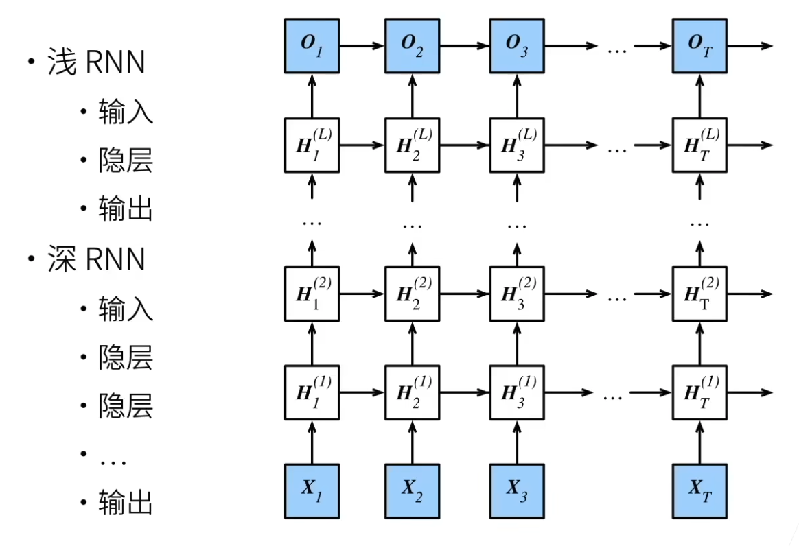
• 每个隐藏层之间传递的是$H_t$

$$ a^{[l]}_t = g(W_a^{[l]}a^{[l-1]}_t + b_a^{[l]}) $$

$$ y_t = g(W_y[a^{[l]}_t, a^{[l-1]}_t, \cdots, a^{[1]}_t] + b_y) $$

• $a^{[l]}_t$ 是第$l$层的隐藏状态
• $W_a^{[l]}$ 是第$l$层的权重
• $b_a^{[l]}$ 是第$l$层的偏置
• $y_t$ 是输出
• $W_y$ 是输出权重
• $b_y$ 是输出偏置

$$ H_t^1 = f_1(H_{t-1}^1, x_t) $$

$$ H_t^2 = f_2(H_t^1, H_{t-1}^2, x_t) $$

$$ H_t^n = f_n(H_t^{n-1}, H_{t-1}^n, x_t) $$

$$ y_t = O_t = g(W_yH_t + b_y) $$

17.6 双向RNN

• 双向RNN使用两个隐藏层，一个隐藏层从前往后传递，一个隐藏层从后往前传递

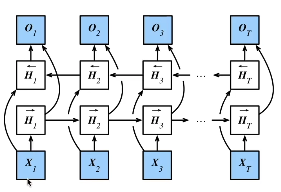
$$ \overrightarrow{a}t = \overrightarrow{a}{t-1} + \overrightarrow{a}_t $$

$$ \overleftarrow{a}t = \overleftarrow{a}{t+1} + \overleftarrow{a}_t $$

$$ H_t = [\overrightarrow{a}_t, \overleftarrow{a}_t] $$

$$ y_t = g(W_yH_t + b_y) $$

18. Attention is all you need

18.1 注意力机制

• 关注需要关注的东西

  • 直观理解，在文字向量中，文字在不同语境下有不同的含义，注意力的作用就是调整文字向量，让它局限于它应该使用的意思

• 卷积、全链接、池化层都只考虑不随意线索

• 注意力机制则显式的考虑了随意线索

  • 随意线索被称为查询 query
  • 需要考虑的线索被称为键 key
  • 需要考虑的线索被称为值 value

• 在RNN的每次计算中，传入的x并非是原始的x，而是x的加权和

18.1.1 非参注意力池化层

• 给定数据（x_i,y_i）,i=1,2,…,n
• 平均池化 $f(x) = \frac{1}{n}\sum_{i=1}^{n}y_i$
• 或Nadaraya-Watson核回归 $f(x) = \sum_{i=1}^{n}\frac{K(x-x_i)}{\sum_{j=1}^{n}K(x-x_j)}y_i$
  • 核函数$K$满足$\int_{-\infty}^{\infty}K(u)du=1$
  • $K(u)=\frac{1}{\sqrt{2\pi}}e^{-\frac{u^2}{2}}$
  • 类似于softmax
  • $f(x)=\sum_{i=1}^{n}softmax(-\frac{1}{2}((x-x_i)w)^2)y_i$
    • $w$是可学习参数
    • $-1/2((x-x_i)w)^2$是高斯函数
    • $-\frac{1}{2}(x-x_i)^2$是注意力分数

$$ y_t = \sum_{i=1}^{n} \alpha_{ti} x_i $$

$$ \alpha_{ti} = \frac{e^{x_i^Tx_t}}{\sum_{j=1}^{n} e^{x_i^Tx_t}} $$

18.1.2 注意力分数

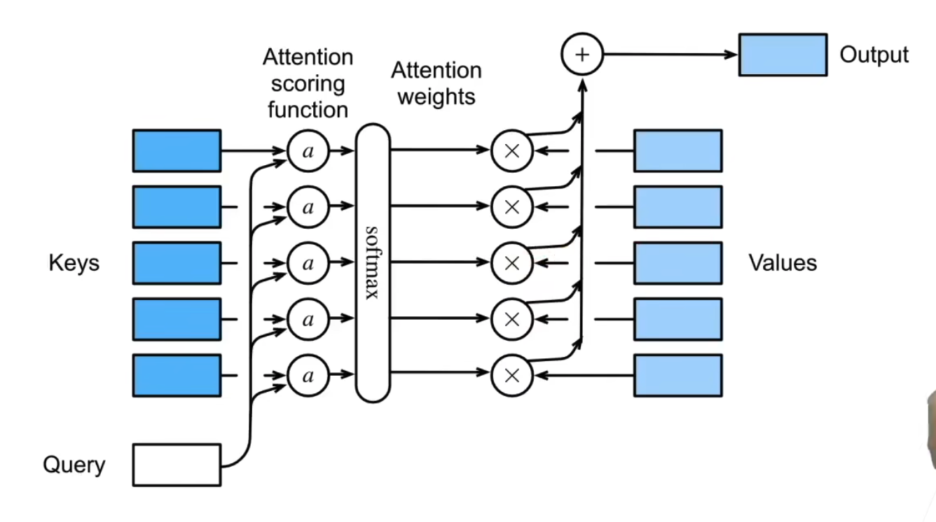
$$ attention_score(q,k,v) = softmax(\frac{q^Tk}{\sqrt{d}})v $$

• $q$ 是查询

• $k$ 是键

• $v$ 是值

• $d$ 是查询和键的维度

• 注意力分数通过动态权重分配和多维度交互，使模型能够：

  • 捕捉局部与全局依赖，突破序列长度限制。
  • 融合多视角特征，提升语义理解能力。
  • 提供可解释性，辅助模型分析与优化。
  • 灵活适配不同任务（如掩码、稀疏化、跨模态）。
  • 其设计平衡了表达能力与计算效率，成为现代深度学习模型（如Transformer、BERT、GPT）的核心组件。

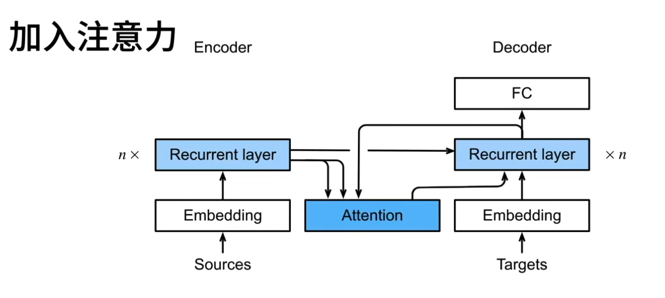
18.1.3 使用注意力机制的seq2seq

• 原本是将最后一个隐藏状态作为解码器的输入，这样的上下文信息有限，一旦句子过长可能会遗忘信息
• 因此在翻译时翻译时，关注对应部分

• 相当于是在每次更新状态时使用编码器生成kv，在用解码器获取q，然后使用注意力机制获取上下文信息

• 注意力机制的核心是让解码器在生成每个词时，能动态“回头看”编码器的相关信息（通过 Q 与 K 的交互），再基于 V 的加权信息辅助预测。这种机制大幅提升了模型对长序列和复杂对齐关系的建模能力。

• 编码器-解码器架构

• 编码器将输入序列编码为上下文向量

  • 生成每个时间步的隐藏状态​（例如，LSTM的输出）。这些隐藏状态直接作为 ​K（键）​​ 和 ​V（值）​。
  • 在标准注意力机制中，K 和 V 通常是同一个东西（即编码器的隐藏状态），但某些变体（如Transformer）可能通过线性变换将它们投影到不同空间。

• 解码器使用上下文向量生成输出序列

  • 解码器的当前隐藏状态​（例如，上一时间步的输出生成的隐藏状态）作为 ​Q（查询）​
  • 注意力机制通过计算 Q 和所有 K 的相似度（如点积、加性注意力等），得到注意力权重，再对 V 加权求和，生成动态上下文向量。

• 注意力机制在解码器中使用，帮助解码器关注输入序列的特定部分

  • 基于时间步生成多对kqv，然后使用注意力机制获取上下文信息

18.2 多头注意力

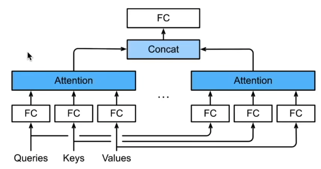
• 普通注意力机制，理解为对语句中的特征进行加权融合
• 多头注意力机制可以理解为多组独立的观察视角，捕捉不同角度的语义信息
• 体现为将输入的特征进行多组线性变换，然后使用注意力机制进行融合，形成同等维度的输出注意力

18.3 自注意力

自注意力机制是一种注意力机制，它使用相同的输入来计算注意力分数

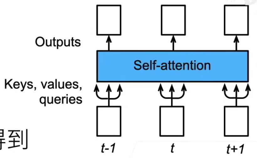
$$ self-attention(X) = softmax(\frac{XW^Q(XW^K)^T}{\sqrt{d}})XW^V $$

• 基本注意力：动态关注外部序列（如编码器到解码器），但关联范围受限。
• 自注意力：动态关注内部全局关系，直接建模序列内部任意位置的依赖。（直接把编码解码器融合在一起）
• 共同点：两者均通过数据自动学习权重，而非人为定义；差异在于应用场景和关联范围。
• 核心创新：自注意力通过全局并行计算，突破了传统模型的归纳偏置（如局部性、顺序性），使模型更灵活地捕捉复杂依赖关系。

18.4 Transformer

• 前馈神经网络

  • 直观理解，就是全连接层，实现了1x1的卷积核对维度进行变换的能力
  • 基于位置的前馈神经网络
    • (b,n,d) -> (bn,d)
    • 作用于两个全链接层

• 预测时

  • 预测第t+1个词
  • 解码器输入前t个预测值
    • 前t个作为k，v，第t个预测值还被作为q